Lambda Calculus
Lambda calculus is an alternative way to model turning machines.
Definitions:
- Variables: Denoted by ordinary lower case letters: \(x, y, f, g, ...\)
- Abstractons: Denoted as \(\lambda \langle var\rangle.\langle body \rangle\) (e.g. \((\lambda x.x)\) is the identity function)
- Applications: \(AB\), where \(A\) and \(B\) is a term (similar to Haskell's
f a, wherefis a function)- Terms: a term is constructed using the items above
A variable is bound, if it is enclosed by a lambda and the lambda binds the term. On the other side, a free variable isn't defined by a lambda.
More formal, it can be defined by introducing a function \(free(A)\), which returns a set of the free variables of the term \(A\):
- \(free(A)=\{\}\), if \(A\) is a constant
- \(free(A)=\{A\}\), if \(A\) is a variable
- \(free(B C) = free(A) \cup free(B)\), given \(A\) and \(B\) is a term
- \(free(\lambda x.B)=free(B) \setminus \{x\}\)
A \(\lambda\) term with no free variables are called combinator
The following are examples how associty works:
A B C = ((A B) C)\x.A B C = \x.((A B) C)\x y.A B \u.A = \x y.((A B)(\u.A)
An interesting note, is that part of the reason why conditionals work, is because lambda calculus uses call-by-name semantics. In languages, like Python or Scheme, this won't work, since these languages will evaluate all parameters before calling the function.
Reductions
There are three ways to manipulate a term:
- \(\alpha\)-conversion
- \(\beta\)-reduction
- \(\eta\)-reduction (eta-reduction) / \(\delta\)-reduction
Lambda calculus uses normal-order "calls" functions, meaning that parameters are not evaluated before applying them to a function. Compare this with the applicative-order, where the parameters are evaluated before calling the function. This is the order "normal" programming languages use.
Reductions are done until no more reductions \(\beta\)-reductions are possible. This form is called \(\beta\)-normal form.
One important note: Reducing doesn't necessarily mean that term becomes smaller.
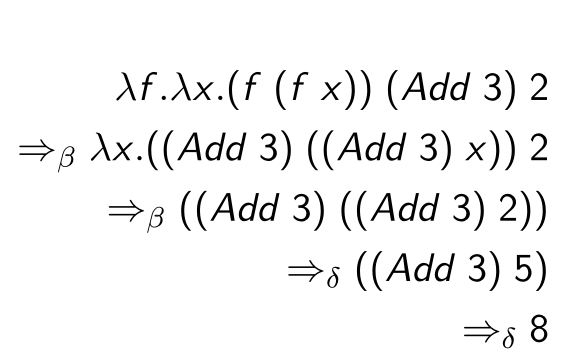
The following is an example of how to calculate with reductions:
\(\alpha\)-conversion
The \(\alpha\)-conversion says that terms can be renamed: $$ \lambda x.A \Rightarrow_\alpha \lambda y.A[x:=y] $$
\(\beta\)-reduction
However, this is only allowed, if during this process no free variable is bound. For example, the following wouldn't be valid: $$ \begin{align}
\end{align}
$$
The following is an example:
$$
\begin{align}
\DeclareMathOperator{\add}{add}
& (((\lambda fgx.(f (g x)) (\add 3)) (\add 2)) 0) \
= & (((\lambda gx.(f (g x)) [f := (\add 3)] (\add 2)) 0) = (((\lambda gx.((\add 3) (g x))) (\add 2)) 0) \
= & ((\lambda x.((\add 3) (g x)) [g := (\add 2)]) 0) = ((\lambda x.((\add 3) ((\add 2) x))) 0) \
= & ((\add 3) ((\add 2) x) 0 [x := 0]) = ((\add 3) ((\add 2) 0) \
\end{align}
$$
\(\eta\)-reduction/\(\delta\)-reduction
Reducuction-Strategies
- Normal Order Reduction ("von aussen nach innen") The term is evaluated from left to right. This is basically lazy-evaluation.
- Applicative Order Reduction ("von innen nach aussen") The most inner term is evaluated first. This is equivalent to strict evaluation.
The term above can be solved, if reduced with the normal reduction . If reduced with the applicative order reduction, then this fails.
However, independent of which reduction strategies was chosen, if there is a result, it will be equivalent. The only difference between the reduction strategies is that it might not complete.
Examples
While-True
The term above is a fix-point and when reduced will yield the same term again.
Y-Combinator
The term above is the Y-combinator, which enables recursions in the \(\lambda\)-calculus.
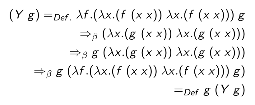
Note: the Y-combinator only works with the normal order reduction (lazy-evaluation).