Linear Regression
A linear function, adjusted to a set of results, can be used to predict the result of other input values. The function takes the following form:
Logistic regression can be found at Classification in the chapter Logistic Regression.
Assumption of Linear Regression
The following assumptions are made for the input and output of a linear regression:
- Linearity: the input and output correlat linearly
- Independence: the outcome of one sample does not affect the outcome of a different sample
- Normality: Errors should be normally distributed (large deviations from the mean should be more unlikely)
- Equality of Variance: Error distribution should be the same for all input values
Cost Function
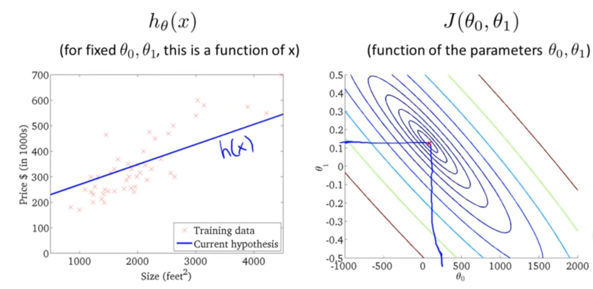
To find a fitting function \(h_\theta\), we want to minimise \(\frac{1}{2m}\sum^m_{i=0}(h_\theta(x_i)-y_i)^2\) (halve of the average of the summed error squared). More formally, this is named a cost function: $$ J(\theta_0, \theta_1)=\frac 1 {2m}\sum^m_{i=0}(h_\theta(x_i)-y_i)^2 $$ This cost function is also called the squared error function.
Cost functions can be plotted as a contour graph. In the example below, the marked spot on the contour plot corresponds with the plot of \(h_\theta(x)\).
The cost function is always convex.
Gradient Descent
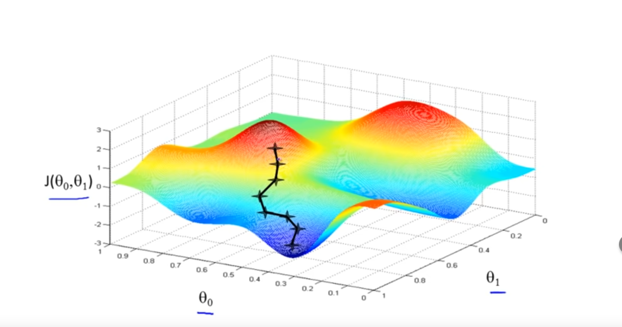
Gradient decent is a general algorithm to find a local minimum of a function.
The algorithm starts at a guess and then, as long as possible, moves the current position to a location where the function is lower. This is repeated, as long as there is a lower position. $$ \begin{flalign} &\text{repeate} \text{ until convergence {} && \ & \hspace{2em} temp_0 := \theta_0-\alpha \frac{\partial}{\partial \theta_0}J(\theta_0, \theta_1)\ & \hspace{2em} temp_1 := \theta_1-\alpha \frac{\partial}{\partial \theta_1}J(\theta_0, \theta_1)\ & \hspace{2em}\theta_0 := temp_0\ & \hspace{2em}\theta_1 := temp_1\ &\text{}} \ \end{flalign} $$ Importantly, the code above updates \(\theta_0\) and \(\theta_1\) simultaneously. \(\alpha\) is the learning rate. It dictates the step size. However, even when \(\alpha\) is fixed, gradient descent can still converge to a local minimum as the derivation will get smaller and smaller when the algorithm gets closer to a local minimum.
The code above can easily be extended to support as many variables as needed.
Cost Function and Gradient Descent
To use the gradient descent algorithm to find the local minimum of the cost function \(J\), the partial derivation of \(J\) for \(\theta_0\) and \(\theta_1\) is needed. Luckily, these are straight forward: $$ \begin{align} \frac{\partial}{\partial \theta_0}J(\theta_0, \theta_1 &= \frac{\partial}{\partial \theta_0} \left(\frac{1}{2m}\sum^m_{i=1}(h_\theta(x_i)-y_i)^2\right) =\frac{1}{m}\sum^m_{i=1}(h_\theta(x_i)-y_i)\
\frac{\partial}{\partial \theta_1}J(\theta_0, \theta_1 &= \frac{\partial}{\partial \theta_1} \left(\frac{1}{2m}\sum^m_{i=1}(h_\theta(x_i)-y_i)^2\right) =\frac{1}{m}\sum^m_{i=1}(h_\theta(x_i)-y_i)\cdot x_i \end{align} $$
These partial derivations can be plugged in the algorithm of gradient descent.
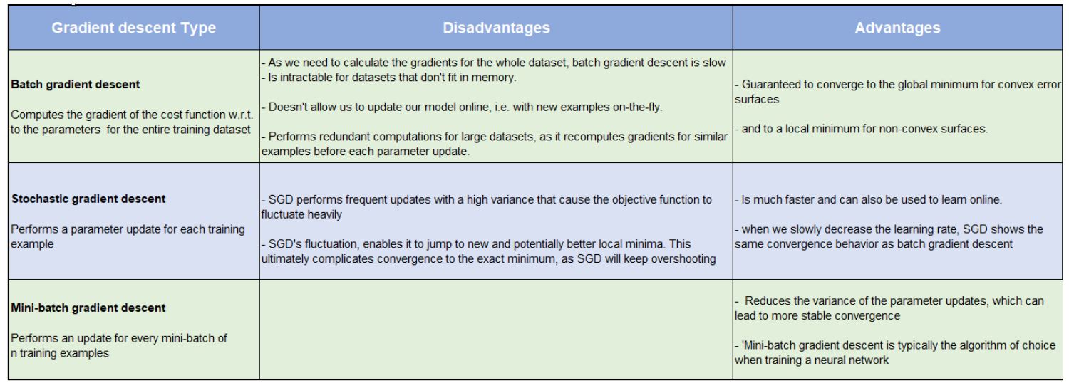
Gradient Descent Mode
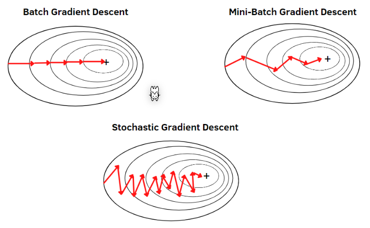
There are multiple "modes" how the gradient descent can function:
-
Batch Gradient Descent Every sample is used to calculate the incline
-
Mini-Batch Gradient Descent
\(n\) random samples are used to calculate the incline
- Stochastic Gradient Descent
One random sample is used to calculate the incline
Multivariate Linear Regression
If there are more than one feature, the hypotheses has to be adjusted to reflect this: $$ h_\theta(\vec x)=\theta_0x_0 + \theta_1x_1 + \theta_2x_2 + ... + \theta_nx_n $$ \(x_0\) is always defined as \(1\). This simplifies \(h_\theta(\vec x)\) as all terms are the "same".
This can also be written with vectors: $$ \vec x = \begin{pmatrix} x_0 \ x_1 \ x_2 \ ... \ x_n \end{pmatrix} \ \vec \theta = \begin{pmatrix} \theta_0 \ \theta_1 \ \theta_2 \ ... \ \theta_n \end{pmatrix} \ h_\theta(\vec x)=\theta_0x_0 + \theta_1x_1 + \theta_2x_2 + ... + \theta_nx_n = \vec\theta^T \cdot \vec x $$ The vectors \(\vec x\) and \(\vec \theta\) have the size \(n+1\), where \(n\) is the number of features. $$ \begin{flalign} &\text{repeate} \text{ until convergence {} && \ & \hspace{2em} \theta_j := \theta_j-\alpha \frac{\partial}{\partial \theta_0}J(\theta_0, \theta_1) =\theta_j-\alpha \frac{1}{m}(h_\theta(x^{(i)}) - y^{(i)})\cdot x_j^{(i)}\ &\hspace{2em}\text{for } j \in {0, 1, ..., n+1}\ &\hspace{2em} \text{(simultaneously update } \theta_j \text{)}\
&\text{}} \ \end{flalign} $$
Gradient Descent with Matrices
Gradient descent can also be implemented with matrices. For this, the derivation can be calculated with the following: $$ \frac{\part J(\vec \theta)}{\part \vec \theta}=-2X^T\vec y + 2X^TX\vec \theta $$ Then \(\vec \theta\) can be updated with the following: $$ \vec \theta_{i+1} = \vec \theta_{i} - \alpha\frac{\part J(\vec \theta_i)}{\part \vec \theta_i} $$
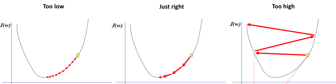
Learning Rate
\(\alpha\) is the learning rate. If it is too low, the steps are very small. If they are high, gradient descent jumps around.
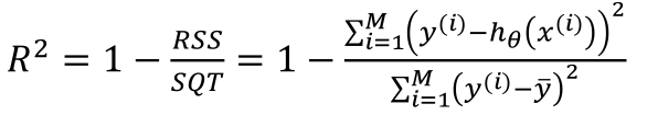
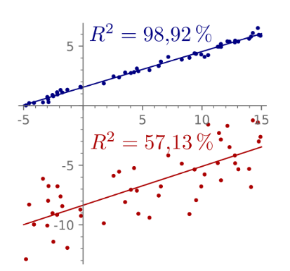
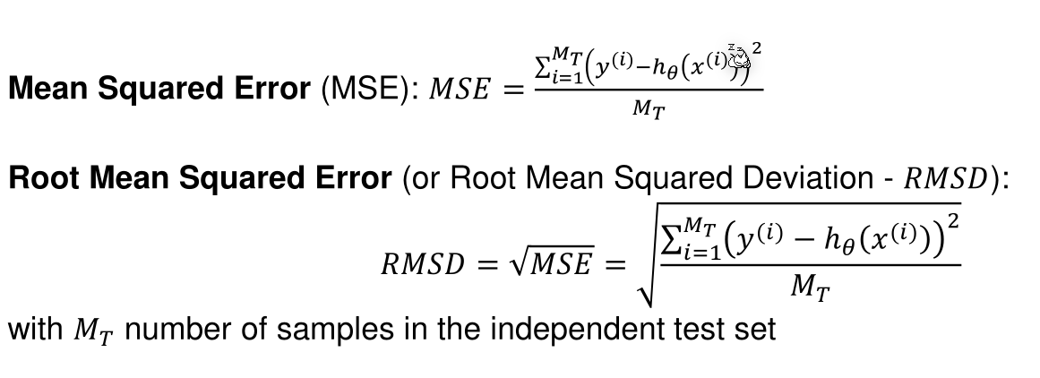
Evaluation Metrics for Linear Regression
\(R^2\) is the percentage of samples which can be explained by the regression.