Data

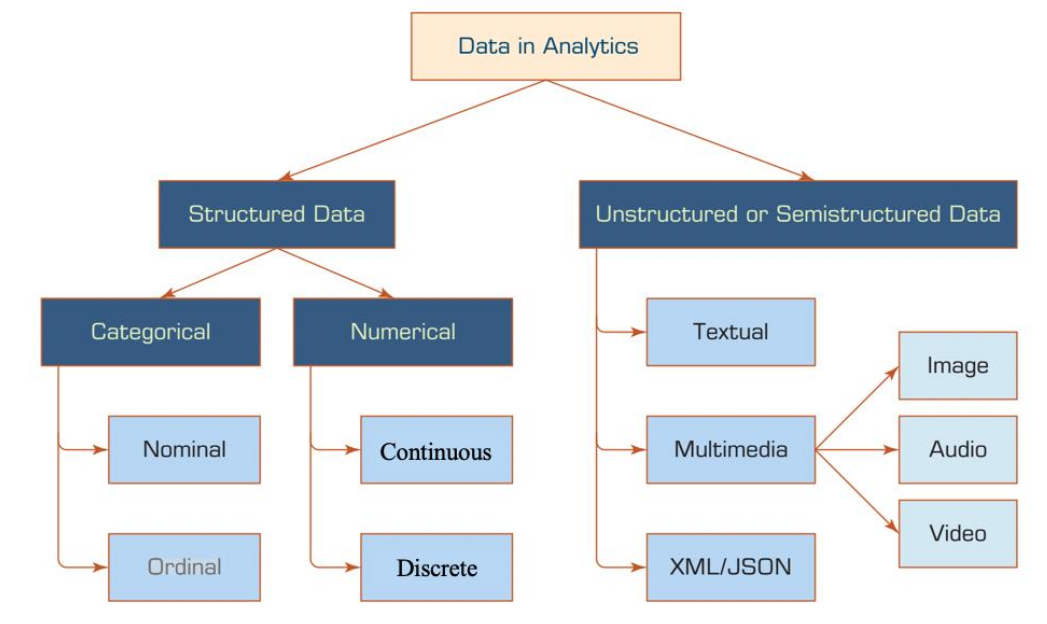
Structured Data Structured data has a fixed data model
Categorical Discretete data like labels
- Nominal Discrete data which cannot be ordered (e.g. labels)
- Oridnal Discrete data which can be ordered
Numerical Numerical data
- Continuous There are no discrete steps (e.g. floating-points)
- Discrete There are discrete steps (e.g. whole integers)
Unstructured/Semi-structured Data Unstructured and semi-structured data does not have a fixed data model. XML and JSON are often classified as semi-structured data

The actual encoding does not effect how the data can be analysed. Even if some data, which physically is continuous, is stored discrete, it can still be analysed as if it was continuous.

Encoding Categorical Data

With encoding categorical data can be encoded with a numeric representation

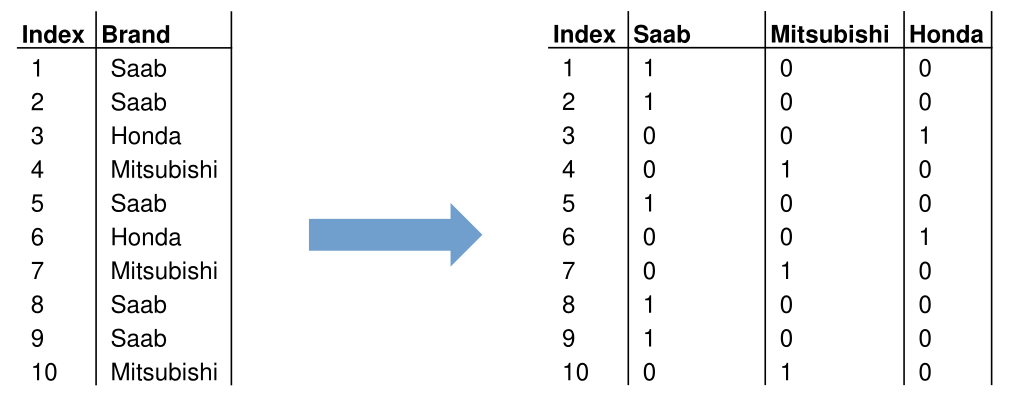
One-Hot Encoding For every category a new boolean variable is being created. If true then the category is present, if false the category is absent
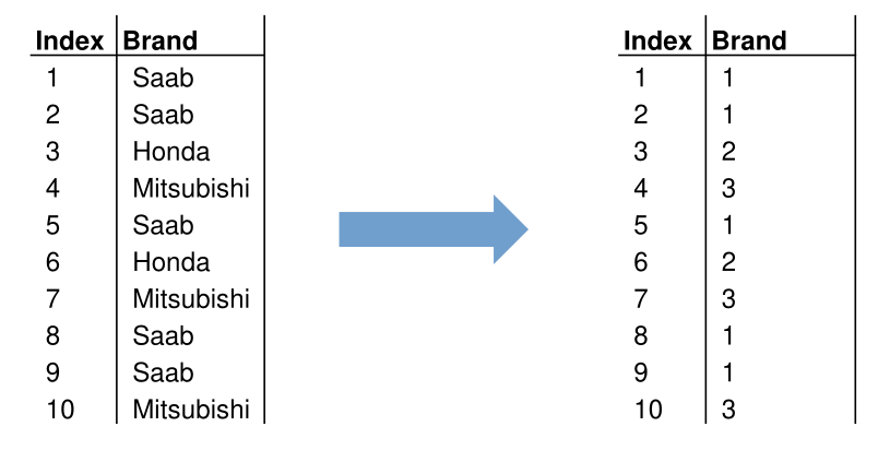
Label Encoding Every category is associated with an integer value
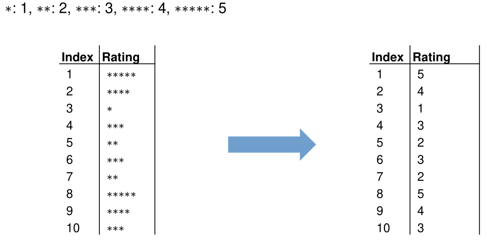
Ordinal Encoding Associate every category an integer based on its order. This only works for ordinal data

Design Matrix (Daten Matrix)

The data can be expressed by a $N\times D$ matrix with numerical values, where $N$ is the amount of samples and $D$ the amount of variables/features.

\[ X_{N\times D}= \begin{pmatrix} x_1^{(1)} & x_2^{(1)} & ... & x_D^{(1)} \\ x_1^{(2)} & x_2^{(2)} & ... & x_D^{(2)} \\ ... & ... & ... & ... \\ x_1^{(N)} & x_2^{(N)} & ... & x_D^{(N)} \\ \end{pmatrix} $$ The following vector $x^{(n)}$ expresses all variables of the $n$-th sample and is equivalent to a row of the design matrix $$ x^{(n)}= \begin{pmatrix} x_1^{(n)} \\ x_2^{(n)} \\ ... \\ x_D^{(n)} \\ \end{pmatrix} \]

Typical Data Processing

As data will rarely be in the correct format and quality needed for analysis, the following tasks often will be performed to bring the data up to the required standard.

Data integration/consolidation Collect and merge the data from multiple sources
Data cleaning Remove and modifying incorrect data
Data transformations Normalize, descretize and aggregate data
Data reduction Reduce data by removing samples and/or attributes

Data Cleaning

Detect (near) duplicates Duplicate numeric values can be detected with the distance/similarity of the feature vectors. Text duplicates can be detected with the Levinstein-Distance.
Missing values Missing values can be replaced by measures of central tendency, like the average or median, replace the value with a fixed value (like -1), fix manually or simply remove the row entirely.
Detect outliers Outliers should be removed as they are usually a result of an error
Smoothing Smoothing eliminates noise and can make patterns more noticeable. There are different methods
Equal-width Binning The range of the data is divided in $N$ bins of equal size. Outliers can dominate the result when only few data points are in a bin. Each bin is replaced by the mean or the closest boundary value.
Equal-depth Binning There are still $N$ bins but each bin has the same number of samples. Each bin is replaced by the mean or the closest boundary value.
Smoothing by bin boundaries replace each value by closest boundary value [24, 28, 29, 35], [41, 41, 44, 45], [46, 48, 49, 54] $\to$ [24, 24, 24, 35], [41, 41, 45, 45], [46, 46, 46, 54]

Feature Scaling

Feature scaling is used to get all data in the same number range since many algorithm perform poorly with different number ranges (e.g. person height between 1.5 and 2.2m, and wheight between 65kg and 80kg)

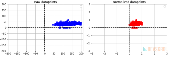
Min-Max Normalisation

This will transform all data points between 0 and 1 $$ x'=\frac{x - \min(x)}{\max(x) - \min(x)} $$

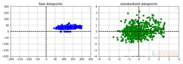
Standardisation

This will transform the data to be distributed around 0 $$ x'=\frac{x-\mu(X)}{\sigma} $$ $\sigma$=Standard Diviation ($\sigma^2$=Varianz)

$\mu$=Average

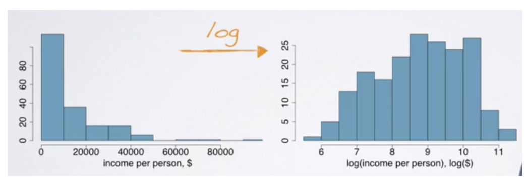
Logarithm

Apply the natural logarithm to the data